ECE 4960: LAB 9 - Mapping
Description
In order to prepare for labs 10-13, a map of the robot area needed to be constructed for future localization and navigation. The lab area had a series of points marked on which the mapping algorithm needed to be ran.
To complete this lab, data was collected at the following waypoints:
[-3, -2]
[-5, -3]
[0, 0]
[0, 3]
[5, 3]
The above waypoints can be seen on the image below, which represents the area that the robot is attempting to map:
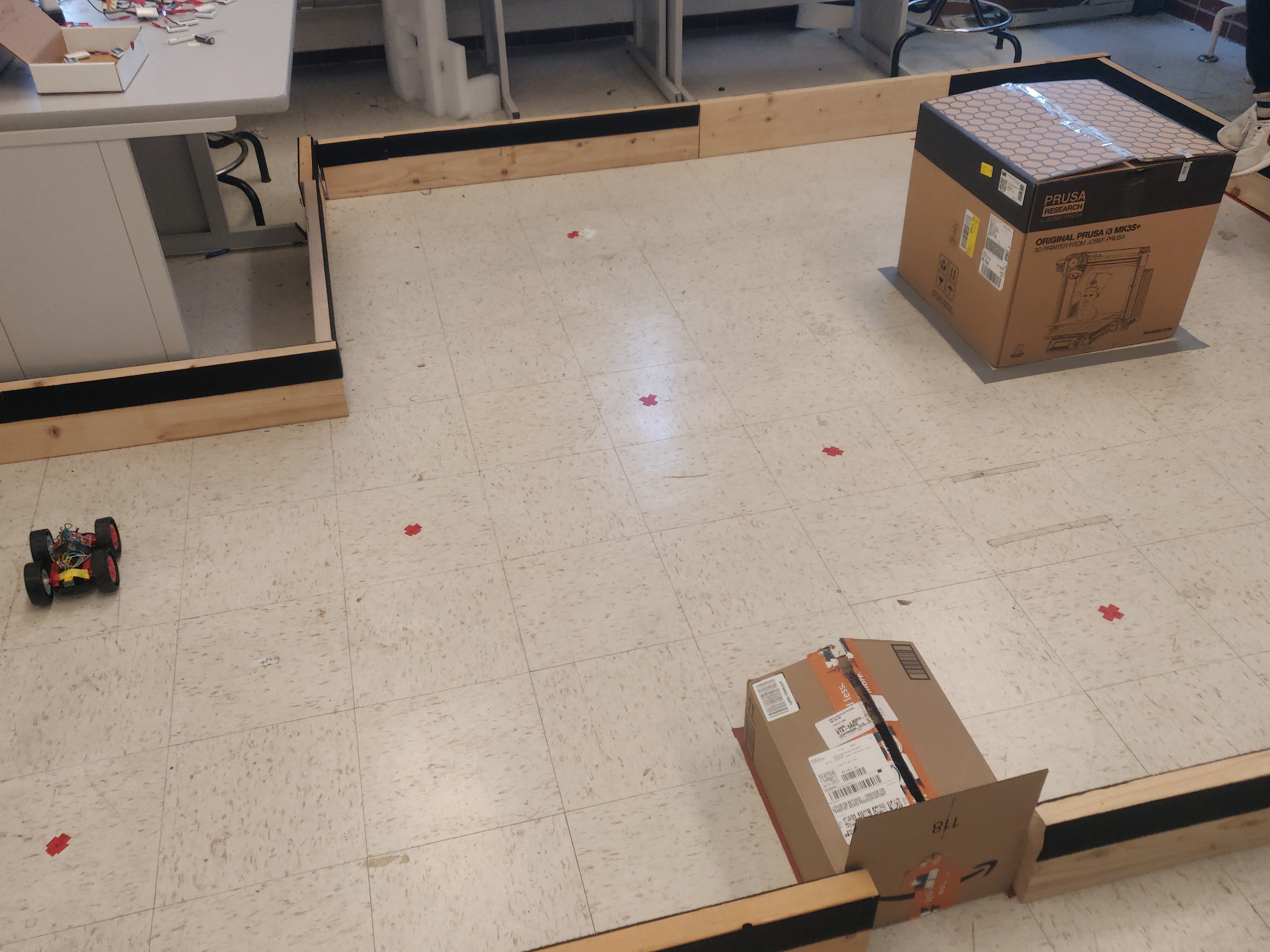
Figure 1: Lab Map Layout
Rotational Control & Data Collection
Out of both available options to complete data collection for this lab, I chose the first option with the robot collecting data while rotating continuously. Instead of limiting data collection to 14 points per location, I gathered more datapoints as to improve the accuracy of the resulting map.
To collect angular and distance data, the robot was rotated while measuring angular rotation. This was done by using the gyroscope Z-axis yaw, in combination with the time delta.
yaw = (myICM.gyrZ() + myICM.gyrZ()*dt*.001)*(.3) + prev_yaw*.7
Where here, dt is the time delta between the current and previous time.
In combination with the rotational data, the distance measurements were also saved:
dist = frontSensor.getDistance();
This resulted into 5 arrays of values with angles, and distance measurements. Below is an example dataset of values collected from the robot:

Figure 2: Example dataset collected from rotation
In order to convert these measurements into actual map locations, the following computations needed to be performed:
1. Convert angle measurements into radians
2. Per location, convert radians + distance measurements into respective X-Y map coordinates
3. Plot points and determine where map lines are found.
Measurement Example: Map Location 1: [5, -3]
This process was first computed for map location 5, -3.
First, the angles were converted to radian measurements:
angle/180.9*np.pi
Next, the x and y location was determine for each reading in the arrays:
x = mapdist[i]*np.cos(map_ang[i]) + 304.5*(5)
y = mapdist[i]*np.sin(map_ang[i]) - 304.5*(3)
As seen above, the x and y points are shifted +5 and -3 respectively to account for the position at which the measurments were takne. Plotting this resulted in the following set of initial map coordinates:
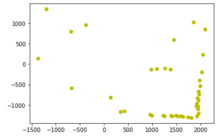
Figure 3: Initial mapping measurements at coordinate 5, -3
Measurements at all 5 locations
The above process was repeated for all 5 map locations, and combined into a single plot. This resulted in the following scatterplot map.
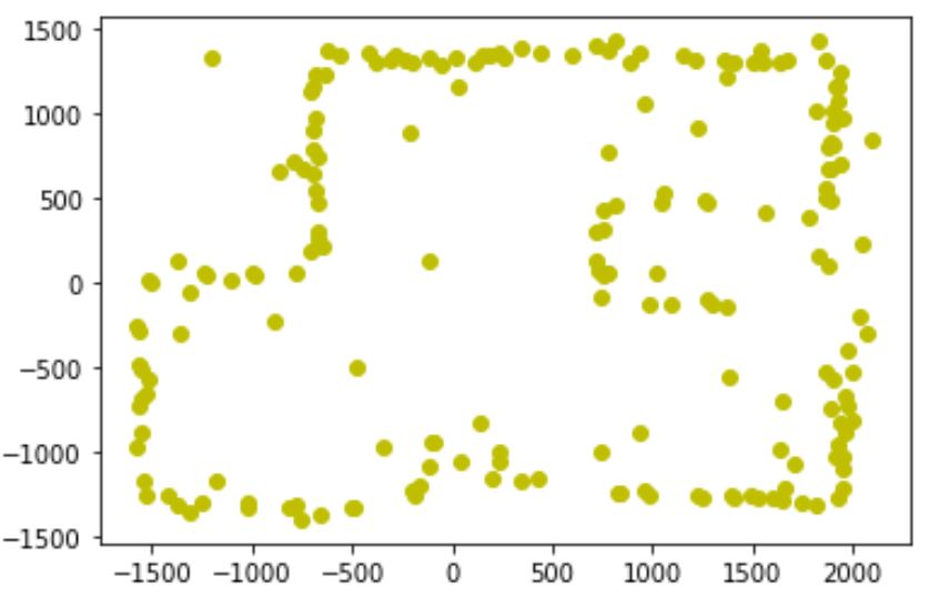
Figure 4: Full mapping measurements at all 5 locations
Constructing the Map
The next part of this lab was to approximate the location of supposed walls in the area, and save them to a list for use in the simulator with lab 10.
According to the plotted configuration of measurements, the following walls were approximated:
walls_x = [1900, 1900, -700, -700, -1550, -1550,-1550, -150, -150, 250, 250, 1900]
walls_y = [-1250, 1300, 1300, 50, 50, -1250, -1250, -1250, -900, -900, -1250, -1250]
square_x = [1400, 750, 750, 750, 1400, 1400]
square_y = [500, 500, -100, -100, -100, 500]
This resulted in the following wall map:
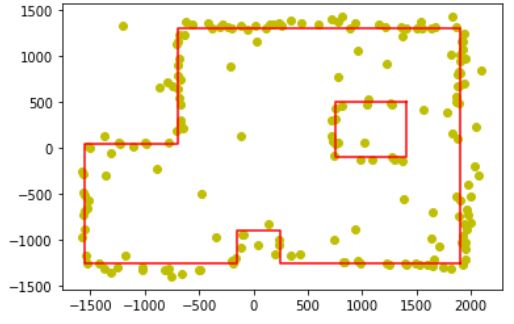
Figure 5: Mapping measurements with approximate wall locations
Removing measurement errors
As a last optional step (moreso for cleanliness/visuals of the map rather than utility), distance measurements representing clear error in comparison with other datapoints were removed from the map.
This was done by clearing and removing any datapoints that were not located on or near one of the drawn walls with the following code:
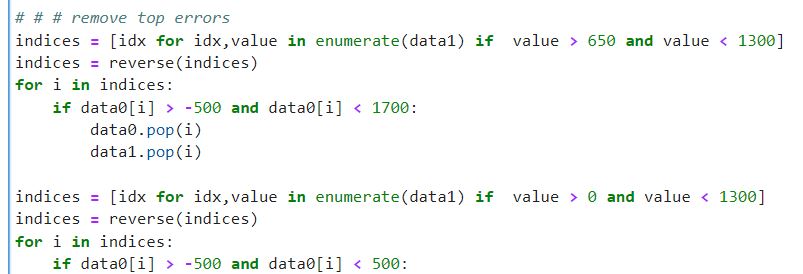
Figure 6: Removing datapoints not located on or near maps
Altogether, this resulted in the following final mapping plot:
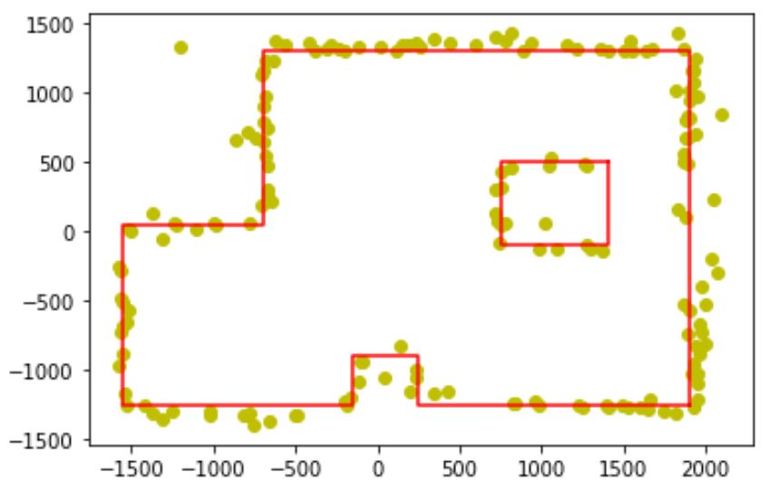
Figure 7: Final plot, Mapping Lab 9
- - - - - This concludes Lab 9- - - - -