ECE 4960: LAB 11 - Grid Localization (Simulator)
Description
The aim of this lab was to complete grid localization within the box2d simulator environment. In this case, a given trajectory was predefined within the simulator, and the goal was to best represent that ground truth trajectory with Bayes Filter localization. For this lab, we were given an initial jupyter notebook with classes an helper functions, as outlined below.
Commander Class
The first set of functions within the simulator environment are packaged within the Commander class. This class allows for interaction with the simulator and plotter, and contains functions to control the robot and retrieve sensor data, plotter functions to plot the map, odometry information, ground truth, and belief, as well as simulator status utility functions.
VirtualRobot Class
The second set of functions within the provided simulator environment are the VirtualRobot class methods. This class acts as a wrapper around the commander class, and similarly controls the robots motion and retrieves sensor information.
Mapper Class
The third set of functions are packaged within the Mapper class. This class holds information related to the grid map, along three dimensions. In our case, the grid map is a 3-d numpy grid with sizes 12 by 9 by 8. It has functions to convert grid indices to world coordinates, and vice versa. It also holds true measurements as a robot should see in a particular cell location. Certain global variables are also defined, such as the grid cells in all dimensions, total observations per cell, and a 4D numpy array with precached views measurements.
BaseLocalization Class
The simulator environment also has a BaseLocalization class. This class holds all grid localization helper functions, to which we will be adding in this lab to complete the Bayes Filter required for localization.
Most important here are the methods get_observation_data(), and gaussian which both play a fundamental role in estimating localization with Bayes Filter.
Getting observation data is required for the sensor model, where in this case we call obs_range_data to retrieve range measurements.
The class also holds variables such as the noise parameters for the sensor, and noise parameters for the rotation and translation of odometry data.
Trajectory Class
Lastly, the simulator environment also holds functions within the trajectory class. This class is simply used to execute a trajectory, which the Bayes localization Filter that we are making in this lab is supposed to approximate.
1. Tasks
a. Prediction Step
The first step in creating the Bayes Filter was to develop the algorithm for the prediction step of the Bayes Filter. This step is shown below, and takes as inputs the current and previous odometry information to use the robot movement information in computing the pose belief. The mathematical description of this step returning bel_bar is shown below:

Figure 1: Bayes Filter Prediction Step
Optimizing Loop Iteration
Considering the large number of operations that need to be performed to update the belief grid, attention was taken to ensure the algorithm would not spend time updating cells which did not affect bel_bar. To do this, while looping over every belief in the 3x3 grid, only cells that had a probability greater than a threshold were updated. This is shown in code below:

Figure 2: Optimizing the Bayes Filter Prediction Step
Motion Model and Bel_bar Calculation
In the case that a cell with non-zero previous belief is found, the algorithm updates that cel with an updated bel_bar. This is done by looping over the full grid and multiplying the previous belief with the motion model output describing the probability of the robot having moved to that new cell in the given timestep.
The motion model was also written for this lab. It takes as input the current and previous pose, and with noise parameters to compute the gaussian probability distribution of the robot's motion. This step is shown below, taking the current pose, previous pose, and control data as inputs:

Figure 3:Motion Model
b. Update Step
Sensor Model
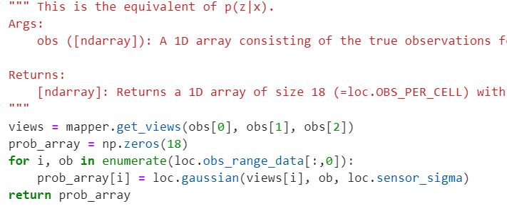
The second step of Bayes Filter Localization is the update step. This step passes as input the true observations of the robot in a given pose on the map, and calculates the probability of each sensor measurement in that pose, outputting them for use in the update step.
The outputted probability array consists of a gaussian probability distribution of the true observations along with the expected observations in that position, given by mapper.get_views.
The developed algorithm for this step is shown below:

Figure 4:Sensor Model
3. Combining Prediction and Update Step in the Bayes Filter
Finally, the prediction and update steps are combined to perform localization with the Bayes Filter. The update step is shown below, returning the new location belief:

Figure 5:Update Step
3. Results
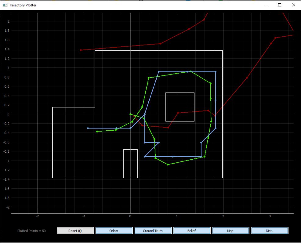
The above algorithm was ran in the simulator, trailing the trajectory defined by the Trajectory class.
The pose belief is calculated after every robot motion by rotating 360 degrees around its axis, collecting range information to compute the sensor model.
In the below video, pose belief is represented in blue, ground truth in green, and odometry information in red.
From the simulator run, we see that the localization algorithm well approximates the true pose, whereas the odometry data
computes the path as being far off what it is expected to be:
Bayes Filter Localization: Simulator
From multiple run iterations, it appears that the robot struggles in accurately localizing in when it turns to the right and reaches the first box osbstalce. The reason for this may be that the object is tall and thin, therefore the robot retrieves measurements showing proximity to the obstacle whereas other measurements do not. The robot seems to most accurately predict pose when objects are relatively far away, such as the upper right area.

Figure 6: Completed Trajectory - Simulator
- - - - - This concludes Lab 11 - - - - -